
Coupling coordination mechanism of higher education and industrial economy: evidence from higher education institutions in Chongqing, China

Analysis of the coupling mechanism between higher education and industrial economy
The level of higher education development is the output of the functioning of the higher education system in a region, which can be reflected by the conditions, scale, quality, and internationalization of higher education (Wu and Liu, 2021). The industrial economy covers all sectors of the national economy, which is mainly reflected by industrial scale, industrial structure, and industrial efficiency (Wang et al., 2022). Higher education and industrial economy mutually reinforce coupling relationships (see Fig. 1).
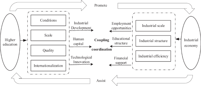
Coupling relationship between higher education and industrial economy.
Higher education for industrial economic development
Higher education can expand the scale, optimize the structure, and enhance the efficiency of the industrial economy. First, higher education expands the industrial scale by directly promoting the development of the tertiary industry. Higher education improves the scientific and cultural level of educated people, thus promoting the development of scientific research, technical services, and high-tech industries (Liu et al., 2024; Zheng et al., 2024). Second, higher education promotes the upgrading of industrial structure by enhancing human capital (Teixeira and Queirós, 2016; Bai et al., 2020). The development of higher education can cultivate more professional talents and optimize the structure of the labor force so that the industrial sector can obtain higher comprehensive quality and promote the upgrading of the industrial structure (Mukhuty et al., 2022). Third, higher education supports industrial efficiency by improving technological innovation (Kong et al., 2022; Zheng et al., 2024). Higher education fosters technological innovation capacity and provides innovation factors for the industrial economy, which is a crucial driver for improving the efficiency of industrial innovation output.
Industrial economy for higher education development
Industrial economic development provides support for higher education. First, industrial economic development offers employment opportunities for higher education by expanding industry scale. Industrial economic development leads to the expansion of industrial scale, enhances the labor demand, and provides high-quality and sufficient jobs for college graduates to optimize the labor market structure (Voumik et al., 2023). Second, industrial economic development leads to optimizing the educational structure by adjusting the industrial structure (AlMalki and Durugbo, 2023). The existing higher education structure makes it difficult for the talents cultivated by colleges and universities to meet the needs of the development of local emerging industries, and the paradoxical phenomenon of “difficult employment” and “labor shortage” coexist. Therefore, to better serve the development of local economies, higher education must scientifically and reasonably adjust its hierarchical, regional, and disciplinary structures. The educational structure will be gradually optimized in this process of adaptation. Third, industrial economic development provides financial support for higher education by improving industrial efficiency (Bertoletti et al., 2022). Industrial economic development will optimize the allocation of resources and enhance economic efficiency, thus increasing local financial income and solving the problem of insufficient funding for education in backward areas.
Measurement of higher education and industrial economy
Indicator system for higher education and industrial economy
Indicator system of higher education (h). Based on the principles of scientificity, hierarchy, representativeness, and operability, combined with the actual situation of the development of higher education in Chongqing, this paper establishes the indicator system of higher education based on the conditions, scale, quality, and internationalization of higher education, respectively (see Table 1).
Industrial economy indicator system (w). In this paper, the industrial economy is divided into three subsystems: industrial scale (w1), industrial structure (w2), and industrial efficiency (w3) (see Table 1). The specific measurements are as follows.
(1) Industrial scale is measured by the value added by each industry.
(2) Industrial structure includes industrial structure rationalization and industrial structure upgrading. The industrial structure rationalization is measured by the inverse of the Theil index, which is calculated as:
$$isr_it=1/TL_it=1/\left[\mathop\sum \limits_j=1^3(Y_itj/Y_it)\mathrmln\left(\fracY_itjY_it\times \fracL_itL_itj\right)\right]$$
(1)
where i is the province; t is the year; isr is the industrial structure rationalization; TL is the Theil index; Y denotes the regional GDP; Yj denotes the value added of industry j; L denotes total employment; and Lj denotes the employment in industry j.
The formula for the industrial structure upgrading is as follows:
$$isu_it=\mathop\sum \limits_j=1^3\fracY_itjY_it\times j$$
(2)
where isu denotes the industrial structure upgrading, Yit and Yitj as above.
(3) Industrial efficiency is calculated using the DEA-Malmquist productivity index method (Chen et al., 2020). The outputs are measured by the value added by the three industries, respectively; the labor input is measured by the year-end employment of the three sectors; and the capital input is estimated by the perpetual inventory method. It should be noted that estimating the capital input of the three industries requires access to the current year’s investment series, depreciation rate, base period capital stock, and fixed asset investment price index. The specific measurements are as follows. ① Current year’s investment series. It is measured by the current year’s fixed asset investment in the three industries. ② Depreciation rate. By weighting the proportion of construction, equipment, and other costs in fixed asset investment from 2013 to 2022, the service life of fixed assets in Chongqing is set at 34 years. Then, assuming a residual value rate of 4%, the average depreciation rate of fixed assets in Chongqing is estimated to be 9.03% (Guo et al., 2023). ③ Base period capital stock. Referring to Young (2003), the formula \(K_0=I_0/(\delta +g)\) is applied. According to the sample period selected in this paper, the base year is determined as 2013, K0 is the base period capital stock, I0 is the comparable fixed asset investment in the base period, δ is the average depreciation rate of capital, and g is the average growth rate of fixed asset investment in Chongqing during the sample period. ④ Fixed asset investment price index. Since the fixed asset investment price index for each industry in Chongqing has not been released, Chongqing’s fixed asset investment price index is used as a substitute.
Methodology for measuring higher education and industrial economy
Based on the indicator system in Table 1, the entropy value method is applied to measure higher education and industrial economy levels, respectively. The steps are as follows.
Since all the indicators are positive, Eq. (3) is used to standardize the data, where max (Xij) and min (Xij) represent the maximum and minimum of variables, i and j represent regions and indicators.
$$x_ij=[X_ij-\,\min (X_ij)]/[\max (X_ij)-\,\min (X_ij)]$$
(3)
Equation (4) calculates the information entropy of each indicator in the composite index system of high-quality economic growth, where n represents the number of regions.
$$d_j=-\,\mathrmln\,\frac1n\mathop\sum \limits_i=1^n\left[\left(x_ij/\mathop\sum \limits_i=1^nx_ij\right)\mathrmln\left(x_ij/\mathop\sum \limits_i=1^nx_ij\right)\right]$$
(4)
Equation (5) is used to determine the weight of each indicator, where m represents the number of indicators.
$$w_j=(1-d_j)/\mathop\sum \limits_j=1^m(1-d_j)$$
(5)
The higher education (h) and industrial economy (w) levels are calculated respectively.
$$h_j(w_j)=\sum _jw_j\left(x_ij/\mathop\sum \limits_i=1^nx_ij\right)$$
(6)
Coupling coordination degree evaluation model
The measurement steps of the coupling coordination degree model are as follows:
Step 1 measures the coupling degree between higher education and industrial economy. Coupling is a principle of physics that refers to the dynamic association of two or more systems that are interdependent, coordinated, and facilitated. The coupling degree records the degree of interaction between system elements. According to the concept of coupling and coefficient model in physics, the coupling degree between higher education and industrial economy (C) is obtained, where 0 ≤ C ≤ 1. When C tends to 0, the systems are detuned. When C tends to 1, the systems are well coupled.
$$C=2\sqrth\times \rmw(h+\rmw)$$
(7)
Step 2, the coupling coordination degree between higher education and industrial economy (D) is measured, better identifying the coordination degree of the interaction coupling between two systems in different regions. T is the comprehensive coordination index, reflecting the synergistic effect between the two systems. α and β are the undetermined coefficients, and set α = β = 0.5.
$$D=\sqrtC\times T,T=\alpha \times h+\beta \times w$$
(8)
The value of D ranges from [0,1], where 0~0.3 is low coordination, 0.3~0.5 is medium coordination, 0.5~0.8 is high coordination, and 0.8~1.0 is extreme coordination.
Empirical model of the coupling mechanism
To test the mutual influence of higher education and the industrial economy, this paper constructs the following model:
$$\rmh_i\rmjt=\alpha _1+\beta _1\rmw_i\rmjt+\mathop\sum \limits_n=1^7\theta _\rmnC_\rmijt+\mu _i\rmj+\eta _t+\varepsilon _i\rmjt$$
(9)
$$\rmw_i\rmjt=\alpha _2+\beta _2\rmh_i\rmjt+\mathop\sum \limits_n=1^7\theta _\rmnC_\rmijt+\mu _i\rmj+\eta _t+\varepsilon _i\rmjt$$
(10)
where h is the higher education level; w is the industrial economy level; β denotes the coefficient of the core explanatory variable on the dependent variable, and θ denotes the coefficient of the control variables on the dependent variable; α is a constant term; i is the higher education institution, j is the district and county in which the higher education institution is located, and t is the year; μ and η denote the individual and time effects, respectively, and ε denotes a random error term. C is a vector of control variables, including the economic development (ed), measured by GDP per capita; government expenditure (ge), measured by the share of general budget expenditure of the local government in GDP; the residents’ consumption (rc), measured by the per capita living consumption expenditure of residents divided by GDP per capita; the financial development (fd), measured by the proportion of deposit and loan balances of financial institutions to GDP; the openness degree (od), measured by the proportion of total imports and exports to GDP; the people’s livelihoods (pl), measured by the per capita disposable income of the residents divided by the per capita GDP; and the public cultural services (pc), measured by the number of books per capita in public libraries.
To examine the impact mechanism of the coupling coordination degree between higher education and industrial economy, this paper further constructs the following empirical model:
$$\rmD_\rmxijt=\alpha _3+\beta _3\rmh_i\rmjt+\beta _3w_\rmxijt+\beta _3{\rmh}_i\rmjt\times w_\rmxijt+\mathop\sum \limits_\rmn=1^7\theta _\rmnC_\rmijt+\mu _i\rmj+\eta _t+\varepsilon _i\rmjt$$
(11)
where Dx represents the coupling coordination degree, which is D, D1, D2, D3 in different models, respectively, indicating the coupling coordination degree between h and w, w1, w2, w3; wx is the independent variable corresponding to the dependent variable Dx, which is w, w1, w2, w3 in different models, respectively, indicating the industrial economy, industrial scale, industrial structure, and industrial efficiency; other symbols are consistent with the above equation. Before the empirical analysis, the data of Chongqing districts and counties from 2013 to 2022 were matched with the data of 63 colleges and universities, with 630 observations. The descriptive statistics of each variable are shown in Table 2.
Data sources
Considering data availability, this paper selects 2013~2022 as the period span. The data for the higher education indicators in Table 1 come from the data related to the 63 colleges and universities of Chongqing in the Chongqing Education Yearbook. The data for the industrial economy indicators in Table 1 is sourced from the Chongqing Statistical Yearbook. The data of control variables in Section 2.4 are from China Statistical Yearbook (County-level) and local statistical yearbooks of Chongqing districts and counties. It should be noted that the missing values are supplemented by linear interpolation, and all variables involving price factors are deflated with 2013 as the base period.
link


